London Landscape programming code

London Landscape: R Code guidance

The London Landscape is an ambitious joint project with MOPAC to map and make available over 150 London crime, demographic and socio-economic datasets in an interactive easy-to-use online format. For more information, see the main page.

Introduction

In order to prepare the datasets for submission as a single file to the dashboarding software Tableau, a large amount of data manipulation is required. This is carried out in the open source software R. Code to carry out this manipulation was written and run in R version 3.2.0 – 64 bit – ‘Full of Ingredients’ using R Studio version 0.98.484.

In order for users to run the code, all but the non-standard Metropolitan Police Service datasets (eg. female victims of violence) and externally calculated datasets (eg. vulnerable locality profile) are available publicly, mainly through the London Datastore. Source datasets require the same column format of Geographic code, Year, and Value. A number of external lookup tables are also used in the process and are supplied below.

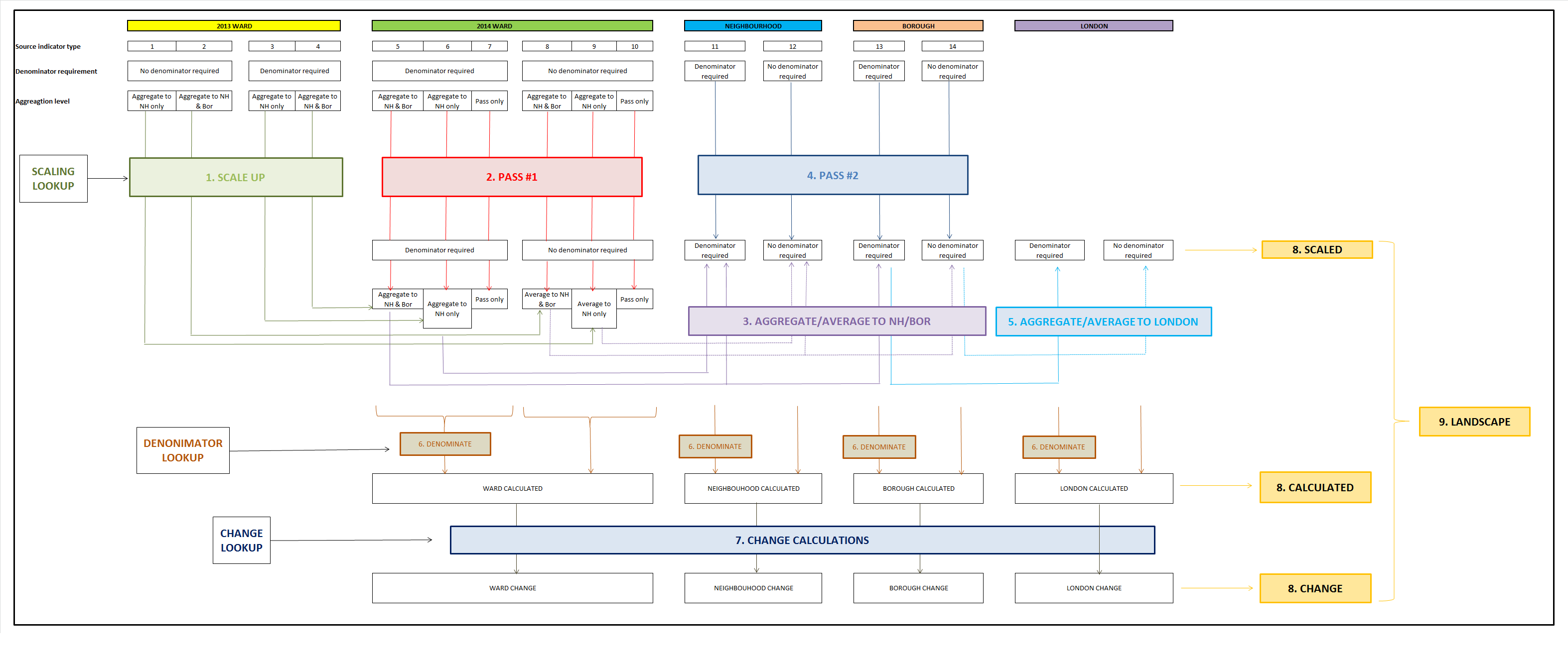
As outlined in the process flowchart there are 9 key stages to the data manipulation, preceded by data staging.

Data Staging	Stage 5: Aggregate/Average #2
Stage 1: Scaling	Stage 6: Denomination
Stage 2: Pass #1	Stage 7: Change
Stage 3: Aggregate/Average #1	Stage 8: Final join #1
Stage 4: Pass #2	Stage 9: Final join #2

The below text outlines the individual processes within each stage, as well as key pieces of relevant R code.

Data Staging

The source data consists of over 100 different emergency service, socio-economic and demographic indicators. Initially the indicators are required to be split into 14 holding folders for later manipulation, dependent on the formats and geographies at which they are available. Each indicator has the same format of geographic code, year and value. NB. some holding folders are empty at this stage, to cover future indicator additions.

Available geography	Calculation type required	Aggregation required	Example
2013 Ward	No denominator required	Neighbourhood only
2013 Ward	No denominator required	Neighbourhood and Borough
2013 Ward	Denominator required	Neighbourhood only	Resident population
2013 Ward	Denominator required	Neighbourhood and Borough	Country of birth
2014 Ward	No denominator required	Neighbourhood only	Fertility rate
2014 Ward	No denominator required	Neighbourhood and Borough	Resident population
2014 Ward	No denominator required	No aggregation required	Pre-calculated vulnerable locality profile
2014 Ward	Denominator required	Neighbourhood only	Drug offences
2014 Ward	Denominator required	Neighbourhood and Borough	Tube footfall
2014 Ward	Denominator required	No aggregation required
Neighbourhood	Denominator required	No aggregation required
Neighbourhood	No denominator required	No aggregation required	Pre-calculated vulnerable locality profile
Borough	Denominator required	No aggregation required	Drug offences
Borough	No denominator required	No aggregation required	House prices

Three lookup tables are used in stages 1, 3 and 6: Scaling lookup , Aggregation lookup , Denominator lookup , and two non-standard R packages are necessary to run the code: dplyr and reshape . See package help for full details.

Stage 1: Scaling

Indicators from the ‘staging’ 2013 ward folders are scaled so that their values represent the geographic areas of the current 2014 ward boundaries. These are placed into identically-named ‘scaled’ 2014 ward holding folders.

# import all files from each ward folder into lists, as well as 2013-to-2014 scaling lookup table 

w13_denom_tonh <- list.files(path = "./Staging/2013 Ward/Denominator required/NH aggregation only", pattern=".csv")
w13_denom_tobor <- list.files(path = "./Staging/2013 Ward/Denominator required/NH & Bor aggregation", pattern=".csv")
w13_nodenom_tonh <- list.files(path = "./Staging/2013 Ward/No denominator required/NH aggregation only", pattern=".csv")
w13_nodenom_tobor <- list.files(path = "./Staging/2013 Ward/No denominator required/NH & Bor aggregation", pattern=".csv")

scaler <- read.csv("./Reference Tables/Ward scaling lookup.csv")

## loop through each of the files within the first list to create the scaled files in the Scaled folders

for(i in 1:length(w13_denom_tonh))
  
{
  setwd("./Staging/2013 Ward/Denominator required/NH aggregation only") 
  dataset <- read.csv(w13_denom_tonh[i]) 
  scaled <- merge(scaler, dataset, by.x=names(scaler)[1], by.y=names(dataset)[1]) 
  scaled[6] <- scaled[3] * scaled[5] 
  scaled_test <- aggregate(scaled[6], by=list(X2014ward=scaled$X2014ward,Year=scaled$Year), FUN=sum) 
  names(scaled_test)[3] <- "Scaled_Value" 
  setwd("./Scaled/2014 Ward/Denominator required/NH aggregation only") 
  write.csv(scaled_test, w13_denom_tonh[i],row.names=FALSE) 
  }

# repeat above loop for remaining 3 ward 2013 file lists, changing both the 'FUN' function to FUN=mean for the 2 lists requiring no denomination, as well as the output file reference.

Stage 2: Pass #1

Indicators from the ‘staging’ 2014 ward folders are passed into the identically-named ‘scaled’ 2014 ward holding folders.

wd14_denom_tonh <- "./Staging/2014 Ward/Denominator required/NH aggregation only/"
target_wd14_denom_tonh <- "./Staging/2014 Ward/Denominator required/NH aggregation only/"
wd14_denom_tonh_files <- list.files(wd14_denom_tonh, "*.csv")
file.copy(file.path(wd14_denom_tonh,wd14_denom_tonh_files), target_wd14_denom_tonh, overwrite=TRUE)

# repeat for each Staging/2014 ward folder

Stage 3: Aggregate/Average #1

To represent indicators not available at neighbourhood and borough levels, ward indicators are aggregated up or averaged depending on the ‘scaled’ folder in which they reside (ie. an indicator in the ‘denominator required / aggregate to neighbourhood and borough’ folder will be raw uncalculated data that can be aggregated up to both neighbourhood and borough levels, whereas one in the ‘no denominator required /average to neighbourhood only’ will have its ward values averaged to represent their parent neighbourhoods). As this is the end of the neighbourhood/borough aggregations, the resultant indicators are placed into either ‘denominator required’ or ‘no denominator required’ neighbourhood or borough folders

# import all files from each ward folder into lists, as well as the geography lookup table (shows relationships between ward-neighbourhood-borough)

wd14_denomtoaggnh <- list.files(path = "./2 Scaled/2014 Ward/Denominator required/NH aggregation only", pattern=".csv")

geog <- read.csv("./Reference Tables/Geography lookup.csv")

# loop through each of the files within the first list

for (i in 1:length(wd14_denomtoaggnh)) {
  
  setwd("./2 Scaled/2014 Ward/Denominator required/NH aggregation only") 
  wd2014 <- read.csv(wd14_denomtoaggnh[i]) 
  wd2014 <- merge(wd2014, geog, by.y=names(geog)[1], by.x=names(wd2014)[1])
  nh_agg <- aggregate(wd2014[3], by=list(Geog=wd2014$NH,Year=wd2014$Year), FUN=sum) 
  names(nh_agg)[3] <- "Aggregated_Value" 
  setwd("./2 Scaled/Neighbourhood/Denominator required/") 
  write.csv(nh_agg, wd14_denomtoaggnh[i], row.names=FALSE) 
  setwd("./2 Scaled/2014 Ward")
  }

# repeat for the remaining 2 'denominator required' folders, and then carry out same process for 3 'no denominator required' folders, substituting FUN=sum for FUN=mean, and amending filenames and output locations appropriately.

Stage 4: Pass #2

Indicators from the ‘staging’ neighbourhood and borough folders are passed into the identically-named ‘scaled’ neighbourhood and borough folders. This gives a complete set of indicators available at neighbourhood and borough levels, separated into ‘denominator required’ or ‘no denominator required’ folders.

# neighbourhood 'denominator required' files (repeat for 'no denominator required' files)

nh_denom <- "./1 Source/Neighbourhood/Denominator required/"
target_denomnh <- "./2 Scaled/Neighbourhood/Denominator required/"
nh_denom_files <- list.files(nh_denom, "*.csv")
file.copy(file.path(nh_denom,nh_denom_files), target_denomnh, overwrite=TRUE)

# borough 'denominator required' files (repeat for 'no denominator required' files)

bor_denom <- "./1 Source/Borough/Denominator required/"
target_denombor <- "./2 Scaled/Borough/Denominator required/"
bor_denom_files <- list.files(bor_denom, "*.csv")
file.copy(file.path(bor_denom,bor_denom_files), target_denombor, overwrite=TRUE)

Stage 5: Aggregate/Average #2

A column defining the data as ‘Base’ data is added; and since a full complement of borough indicators is now available, these indicators can be aggregated up or averaged to a London level, into identically-named ‘denominator required’ or ‘no denominator required’ folders.

# adding of data format column

wd14_denom_nhbor <- list.files(path = "./2 Scaled/2014 Ward/Denominator required/NH & Bor aggregation/", pattern=".csv")

for(i in 1:length(wd14_denom_nhbor))
  
{
  setwd("./2 Scaled/2014 Ward/Denominator required/NH aggregation only/")
    dataset <- read.csv(wd14_denom_nhbor[i])
  dataset[,4] <- substr(wd14_denom_nhbor[i],1,nchar(wd14_denom_nhbor[i])-4)  
  dataset[,5] <- "Base"
  dataset <- dataset[c(1,5,4,2,3)]
  names(dataset) <- c("Geog", "Format Type", "Variable", "Year", "Value")
  write.csv(dataset, wd14_denom_nhbor[i], row.names=FALSE)
  }

# repeat for other 9 'scaled' folders, amending source and output names appropriately

# aggregating/averaging of Borough data to London level (and adding a geography column)

bor_denomtoagglondon <- list.files(path = "./2 Scaled/Borough/Denominator required", pattern=".csv")

for (i in 1:length(bor_denomtoagglondon)) {
  
  setwd("./2 Scaled/Borough/Denominator required")
  bor_agg <- read.csv(bor_denomtoagglondon[i])
  london_agg <- aggregate(bor_agg[5], by=list(Year=bor_agg$Year), FUN=sum)
  london_agg[,3] <- "London"
  london_agg[,4] <- bor_agg[2,2]
  london_agg[,5] <- bor_agg[2,3]
  names(london_agg)[3] <- "Geog"
  names(london_agg)[4] <- "Format Type"
  names(london_agg)[5] <- "Variable"
  london_agg <- london_agg[c(3,4,5,1,2)]
  setwd(".2 Scaled/London/Denominator required")
  write.csv(london_agg, bor_denomtoagglondon[i], row.names=FALSE)
  setwd("/.2 Scaled/Borough/Denominator required")
  }

# repeat for files from borough 'no denominator' folder.

With this complete, a full range of ‘raw’ indicators are available at all geographies from ward to London.

# The files within the 3x 'scaled/denominator required' folders that were used for the aggregating/averaging process can now be moved to a single 'denominator required' folder ready for the denominator calculations. 

ward_denom1 <- "./2 Scaled/2014 Ward/Denominator required/NH & Bor aggregation/"
ward_denom2 <- "./2 Scaled/2014 Ward/Denominator required/NH aggregation only/"
ward_denom3 <- "./2 Scaled/2014 Ward/Denominator required/No aggregation required/"
target_denomward <- "./2 Scaled/2014 Ward/Denominator required/Copy scaled files for calculation/"
ward_denom_files1 <- list.files(ward_denom1, "*.csv")
ward_denom_files2 <- list.files(ward_denom2, "*.csv")
ward_denom_files3 <- list.files(ward_denom3, "*.csv")
file.copy(file.path(ward_denom1,ward_denom_files1), target_denomward, overwrite=TRUE)
file.copy(file.path(ward_denom2,ward_denom_files2), target_denomward, overwrite=TRUE)
file.copy(file.path(ward_denom3,ward_denom_files3), target_denomward, overwrite=TRUE)

# repeat for the files in the 'no denominator required' folders.

Stage 6: Denomination

Denomination indicators (eg. population, housing stock) have been aggregated in the same process above along with the indicators to be displayed in the Landscape. These are now joined together as columns in lookup tables at each of the 4 geographies. A further lookup table is then used to ensure the correct denominators are joined to the indicators in the ‘denominator required’ folders, and that the correct calculation is performed (eg. per capita rate, percentage share). The resultant indicators are placed into a single respective geographic level ‘calculated’ folder. The source denominator indicators are then deleted from the process so that they are not subject to any further calculations. Those indicators that do not require denomination (in the ‘no denomination required’ folders) are simply passed into the relevant geographic ‘calculated’ folder. A column defining these datasets as ‘Calculated’ is also added.

# merge denominator files into single lookup files for each geography

W_Persons <- read.csv("./2 Scaled/2014 Ward/Denominator required/Copy scaled files for calculation/D-Persons.csv")
W_Households <- read.csv("./2 Scaled/2014 Ward/Denominator required/Copy scaled files for calculation/D-Households.csv")
W_Householdspaces <- read.csv("./2 Scaled/2014 Ward/Denominator required/Copy scaled files for calculation/D-Household spaces.csv")
W_Female <- read.csv("./2 Scaled/2014 Ward/Denominator required/Copy scaled files for calculation/D-Female.csv")

#etc

merge1 <- merge(W_Persons, W_Age517, by=c("Geog","Year"), all.x = T, all.y = T)
merge1 <- merge1[c(1,2,3,5,8)]
names(merge1) <- c("Geog","Year", "Format", "Persons", "Age5-17")

merge2 <- merge(merge1, W_Households, by=c("Geog","Year"), all.x = T, all.y = T)
merge2 <- merge2[c(1,2,3,4,5,8)]
names(merge2)[6] <- "Households"

merge3 <- merge(merge2, W_Householdspaces, by=c("Geog","Year"), all.x = T, all.y = T)
merge3 <- merge3[c(1,2,3,4,5,6,9)]
names(merge3)[7] <- "Household Spaces"

merge4 <- merge(merge3, W_Female, by=c("Geog","Year"), all.x = T, all.y = T)
merge4 <- merge4[c(1,2,3,4,5,6,7,10)]
names(merge4)[8] <- "Female"

#etc

write.csv(merge4,"./Reference Tables/R generated/Ward_Denominators.csv", row.names=F)

# repeat for Neighbourhood, Borough and London

# remove individual denominator files 

file.remove("./2 Scaled/2014 Ward/Denominator required/Copy scaled files for calculation/D-Persons.csv")

#etc

# repeat for Neighbourhood, Borough and London files

# for denominating input the list of borough files, the lookup to know which denominator to join to, and the lookup of the denominator data

bor_to_denom <- list.files(path = "./2 Scaled/Borough/Denominator required", pattern=".csv")
Denom_lookup <- read.csv("./Reference Tables/Denominator lookup.csv")
Borough_Denoms <- read.csv("./Reference Tables/R generated/Borough_Denominators.csv")

# start loop of files in folder which carries out join as well as relevant calculation (percentage, rate, per)

for(i in 1:length(bor_to_denom))
  
{
  setwd("./2 Scaled/Borough/Denominator required")
  dataset <- read.csv(bor_to_denom[i])
  dataset_denom_initial <- merge(dataset, Denom_lookup, by= "Variable")
  Denom_type <- dataset_denom_initial[2,7]
  
  Denom1 <- Borough_Denoms[grep("Geog|Year",names(Borough_Denoms)) ]
  Denom2 <- Borough_Denoms[grep(Denom_type,names(Borough_Denoms)) ]
  Denom <- cbind(Denom1,Denom2)
  
  dataset_denom <- merge(dataset_denom_initial,Denom,by= c("Geog","Year"), all.x=TRUE)
  Calc_type <- dataset_denom$Calculation
  Value <- dataset_denom$Value
  Denom_value <- dataset_denom[,8]
  
  Value_temp <- ifelse(Calc_type == 'Rate', Value / (Denom_value/1000), ifelse(Calc_type == 'Percentage', (Value / Denom_value)*100,ifelse(Calc_type == 'Per', Value / Denom_value)))
  dataset_denom[,9] <- Value_temp
  
  names(dataset_denom)[9] <-"Value"
  dataset_denom[,4] <- "Calculated"
  dataset_denom <- dataset_denom[c(1,4,3,2,9)]
  setwd("./3 Calculated/Borough")
  write.csv(dataset_denom, bor_to_denom[i],row.names=FALSE)
  }

# repeat for ward, neighbourhood and London 'denominator required' folders. 

# a move is then required to move all the files from the '2 Scaled/not requiring denomination' folders into the '3 Calculated' folders alongside those that have been moved as a result of the calculations above. 

ward_to_nodenom <- "./2 Scaled/2014 Ward/No denominator required/Copy scaled files for calculation/"
ward_nodenom_files <- list.files(ward_to_nodenom, "*.csv")
target_nodenomward <- "./3 Calculated/Ward/"
file.copy(file.path(ward_to_nodenom,ward_nodenom_files), target_nodenomward, overwrite=TRUE)

# repeat for neighbourhood, borough and London 'no denominator required' folders

# add data format column via loop on above imported files

for(i in 1:length(ward_nodenom_files))
  
{
  setwd("./3 Calculated/Ward/")
  dataset <- read.csv(ward_nodenom_files[i])
  dataset[,2] <- "Calculated"
  write.csv(dataset, ward_nodenom_files[i], row.names=FALSE)
  }

# repeat for neighbourhood, borough and London files

With this complete, a full range of ‘calculated’ indicators are available at all geographies from ward to London.

#Before change calculations can be carried out, those indicators that only have a single years worth of data have to be manually removed

bor_for_change <- "./3 Calculated/Borough/"
target_bor_for_change <- "./3 Calculated/Borough/Variables for change/"
bor_files <- list.files(bor_for_change, "*.csv")
file.copy(file.path(bor_for_change,bor_files), target_bor_for_change, overwrite=TRUE)

file.remove("./3 Calculated/Ward/Variables for change/Household Language English as main language.csv")
file.remove("./3 Calculated/Ward/Variables for change/Household Language English not main language.csv")
file.remove("./3 Calculated/Ward/Variables for change/Passports held Australasia.csv")

#etc

# repeat for ward, neighbourhood, and London files

Stage 7: Change

Using a lookup table assigning each indicator a ‘change group’, the relevant change calculation (eg. one year, five year) is carried out via calculations written in R for each code. The resultant indicators are placed into a single respective geographic level ‘change’ folder.

bor_to_change <- list.files(path = "./3 calculated/Borough/Variables for change", pattern=".csv")
Change_lookup <- read.csv("./Reference Tables/Change lookup.csv")

# start loop which joins the indicator to its change group (eg. Group 1pB) and carries out the relevant calculation from the following list

for(i in 1:length(bor_to_change))
  
{  
  setwd("./3 Calculated/Borough/Variables for change")
  dataset <- read.csv(bor_to_change[i])
  dataset <- melt(dataset, id=c("Geog","Format.Type", "Variable", "Year"))
  dataset_pivot <- cast(dataset, Geog ~ Year)
  dataset_pivot <- cbind(Variable = dataset[1,3],dataset_pivot)
  dataset_merged <- merge(dataset_pivot, Change_lookup, by.y="Variable", by.x="Variable")
  Change_group <- as.character(dataset_merged$Change.Group)
  Change_group <- as.character(Change_group[1])
  
 if(Change_group=='Group 1pB') {
     
     dataset_merged[,6] <- ((dataset_merged[,4] - dataset_merged[,3])/dataset_merged[,3])*100
     names(dataset_merged)[6] <- "2001"
     dataset_merged <- dataset_merged[c(1,2,6)]
     dataset_merged<-melt(dataset_merged,id=c("Geog", "Variable"))
     
 } else if(Change_group=='Group 1pC') {
       
       dataset_merged[,6] <- ((dataset_merged[,4] - dataset_merged[,3])/dataset_merged[,3])*100
       names(dataset_merged)[6] <- "2012"
       dataset_merged <- dataset_merged[c(1,2,6)]
       dataset_merged<-melt(dataset_merged,id=c("Geog", "Variable"))
   
#etc

} else {
   
   dataset_merged[,13] <- ((dataset_merged[,6] - dataset_merged[,5])/dataset_merged[,5])*100
   dataset_merged[,14] <- ((dataset_merged[,7] - dataset_merged[,6])/dataset_merged[,6])*100
   dataset_merged[,15] <- ((dataset_merged[,9] - dataset_merged[,6])/dataset_merged[,6])*100
   names(dataset_merged)[13] <- "2014"
   names(dataset_merged)[14] <- "2020"
   names(dataset_merged)[15] <- "2030"
   dataset_merged <- dataset_merged[c(1,2,13,14,15)]
   dataset_merged<-melt(dataset_merged,id=c("Geog", "Variable"))
   
# add and rename columns
   
 dataset_merged[,5] <- "Change to or from" 
 names(dataset_merged)[5] <- "Format Type"
 dataset_merged <- dataset_merged[c(1,5,2,3,4)]
 names(dataset_merged)[4] <- "Year"
 names(dataset_merged)[5] <- "Value"
 
 setwd("./4 Change/Borough")
 write.csv(dataset_merged, bor_to_change[i],row.names=FALSE)
  }   
   
# repeat for ward, neighbourhood and London files

With this complete, a full range of ‘change’ indicators are available at all geographies from ward to London.

Stage 8: Final join #1

The indicators within the final folders for the ‘raw’ (scaled) data, ‘calculated’ data, and ‘change’ data are merged into 3 separate files with the 3 columns of data for each indicator appended below one another. Columns defining geography, indicator name, and thematic area are added.

# append contents of Scaled folders into 'Base' file

setwd("./2 Scaled/Borough/Denominator required")
file_list <- list.files()
bor_base_merge_denom <- do.call("rbind", lapply(file_list, read.csv, header = TRUE))


setwd(".No denominator required")
file_list <- list.files()
bor_base_merge_nodenom <- do.call("rbind", lapply(file_list, read.csv, header = TRUE))

#etc

Base <- rbind(bor_base_merge_denom,bor_base_merge_nodenom,nh_base_merge_denom,nh_base_merge_nodenom, ward_base_merge_denom,ward_base_merge_nodenom, london_base_merge_denom, london_base_merge_nodenom)

# repeat for Calculated folder contents into "Calculated" file, and Change folder contents into "Change" file

Stage 9: Final join #2

The 3 files are appended below one another, with the addition of columns defining the data format, the indicator metadata hyperlink address (to access from within the Landscape), and the related parent geographic codes for ward and neighbourhood data (for linking between geographies within the Landscape).

# append 3 files created 

All_1 <- rbind(Base,Calc,Change)

# add hyperlink column

All_1[,6] <- tolower(All_1[,3])
All_1[,6] <- gsub(" ", "", All_1[,6], fixed = TRUE)
All_1[,6] <- gsub("-", "", All_1[,6], fixed = TRUE)
All_1[,6] <- gsub(":", "", All_1[,6], fixed = TRUE)
All_1[,6] <- gsub(",", "", All_1[,6], fixed = TRUE)
All_1[,6] <- gsub("(", "", All_1[,6], fixed = TRUE)
All_1[,6] <- gsub(")", "", All_1[,6], fixed = TRUE)
All_1[,6] <- gsub("+", "", All_1[,6], fixed = TRUE)
All_1[,6] <- gsub("/", "", All_1[,6], fixed = TRUE)
All_1[,7] <- tolower(All_1[,2])
All_1[,7] <- gsub(" ", "", All_1[,7], fixed = TRUE)
All_1[,8] <- paste("https://londondatastore-upload.s3.amazonaws.com/londonlandscape/",All_1[,6],All_1                                
                      [,7],".html",sep="")

# merge with Geography lookup table

Geog_Tableau <- read.csv("./Reference Tables/Final Geography lookup for Tableau.csv")
All_2 <- merge(All_1,Geog_Tableau, by.y="Ward.Code", by.x = "Geog")

# merge with Theme lookup table

Theme_lookup <- read.csv("./Theme lookup.csv")
All_3 <- merge(All_2,Theme_lookup, by.y="Variable", by.x = "Variable")

# reorder & rename columns

All_3 <- All_3[c(10,11,12,13,14,15,16,2,9,3,17,1,4,5,8)]
names(All_3) <- c("Level","Borough Code", "Borough Full Name", "Borough Name", "Borough Short", "Neighbourhood Code", "Neighbourhood Name", "Ward Code", "Ward Name",  "Data Type", "Theme", "Variable", "Date", "Value", "Hyperlink")

# change date format

Date_lookup <- read.csv("./Date lookup.csv")
All_4 <- merge(All_3,Date_lookup, by.y="Source", by.x = "Date")
All_4 <- All_4[c(2,3,4,5,6,7,8,9,10,11,12,13,16,14,15)]

# export final csv 

write.csv(All_4, "Source_for_Tableau.csv", row.names=FALSE)

With this complete, a single dataset is available containing all the information required for the Landscape.